Emporia State University
Fall 2011
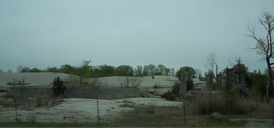
Image of mill remnants at Douthat, Oklahoma. Image by author, 2007.
This webpage was prepared by Gina Manders to fulfill an assignment for ES775 Advanced Image Processing
Emporia State University
Fall 2011
Image of mill remnants at Douthat, Oklahoma. Image by author, 2007.
After downloading Landsat TM datasets for December 9, 1988; December 18, 1997; December 6, 2010; and August 3, 2011, the files were unzipped and imported directly into Idrisi Taiga by selecting File, Import, Government, Landsat and GeoTiff. December images were selected for the benefit of leaf-off conditions in an effort to emphasize areas of soil and chat more clearly. The downloaded datasets were georectified in the UTM projection. Using the Window function (under Reformat), a smaller subscene that focused on the Tar Creek Superfund Site was created and its boundaries were used as a template for creating subscenes with common coordinate boundaries for each band of the dataset for all four years.
Imagery was cropped to just above the Oklahoma/Kansas state line to the north and just below the Oklahoma University Passive Treatment System (OU PTS) in Commerce, Oklahoma to the south. Working images were projected in UTM, zone 15, NAD83 datum. All subsequent Landsat image processing was based on these resampled windows of the TCSS study area.
In an effort to enhance specific features in this closer study area and to emphasize variabilities, color composites of Landsat imagery were created in different light-band combinations for the available datasets. The resolution of six Landsat bands (Bands 1-5 and 7) is 30 meters. Band 6 resolution is 60 meters. The composite module is located under Image Processing/Enhancement:
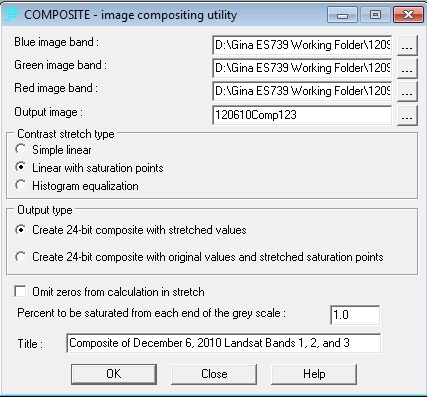
Various composite options were used to seek the most informative combination. Simple linear contrast stretch and contrast stretch were both used and the resulting composites using linear with saturation points, 24-bit composite with stretched values had the best results so that was the combination used for the project.
It was felt since the OU PTS, a series of small connected pools, has been constructed in recent years, it would be helpful to include it to validate whether or not software processes identify changes in the landscape. The datasets were not used for all of the time periods for each GIS process. Rather, most processes were completed on imagery from December 1988 and December 2010. When there were questionable or unusual results, a third time period was added for comparison and/or additional types of processing were completed.
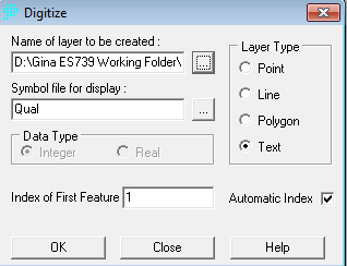
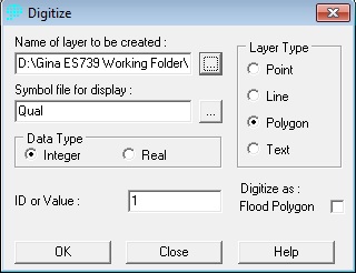
Three vector text layers were prepared through digitizing with the digitize feature in Idrisi for labeling of features on the maps.
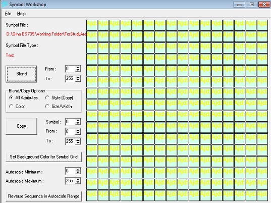
A number of palettes were created in the Idrisi Symbol Workshop for the text.
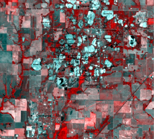
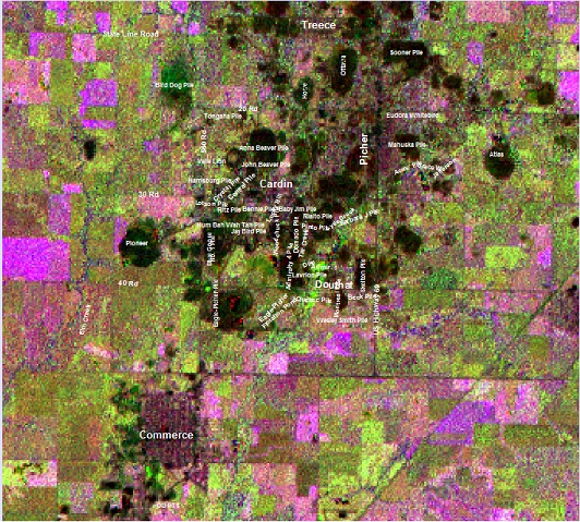
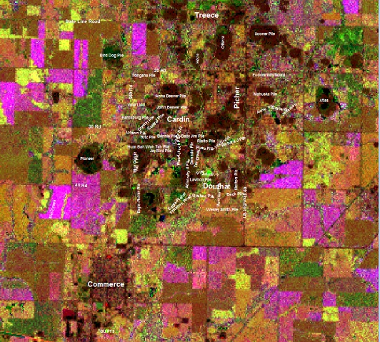
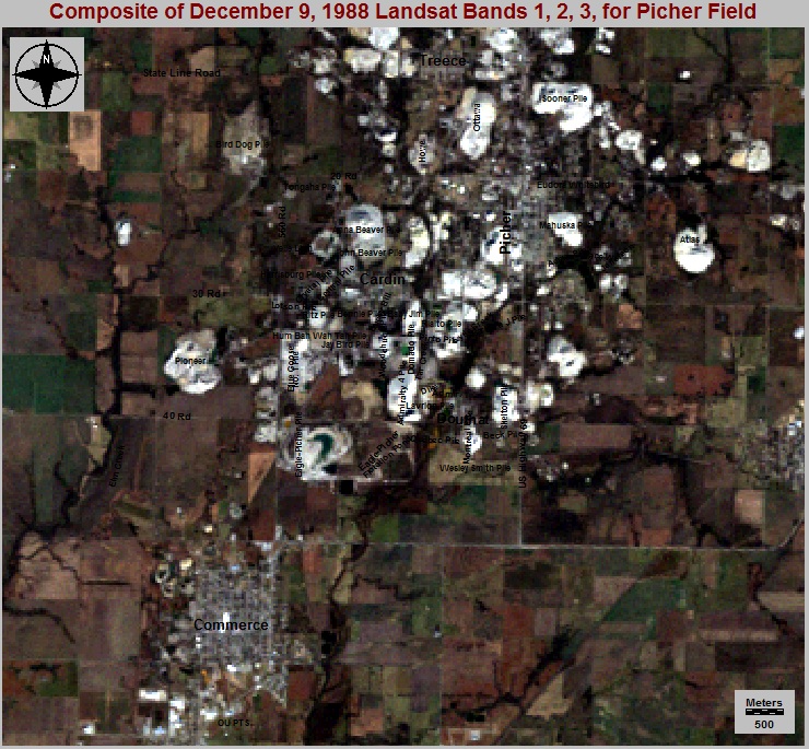
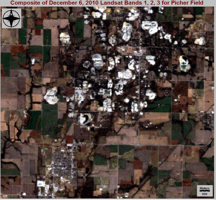
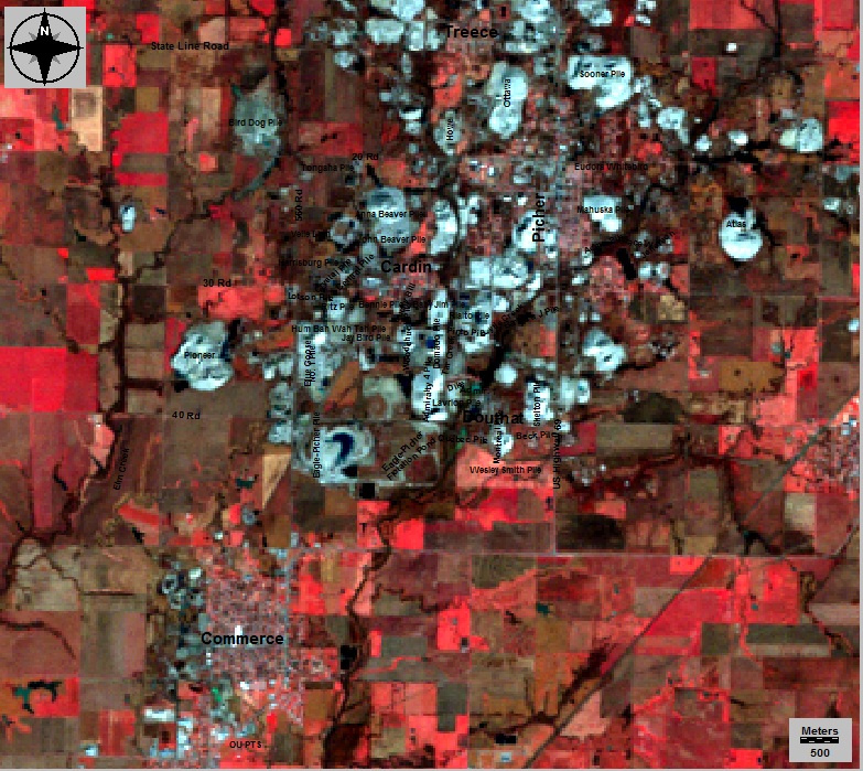
Composite of Bands 1, 2, and 3, color-coded Blue, Green and Red
12/9/88 first image 12/6/10 second image
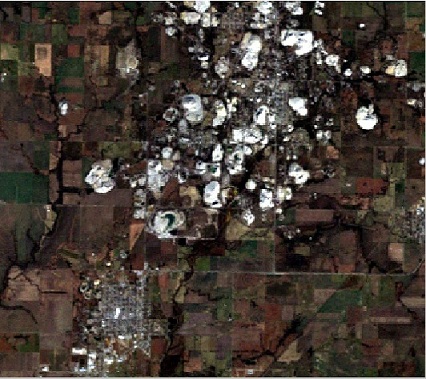
Click here for larger 1988 image Click here for larger 2010 image
Notice the increase in depth of the water in the feature that looks like a crescent. It is simply an area in chat that has less chat and more water now. In addition to changes in locations of crops in fields, there is a noticeable change in the chat pile toward the northeast of the image. According to Ken Luza, Oklahoma University, this pile is now mostly fines but he believes the small layer of chat on top that has spread out makes the pile have stronger reflectance values than in earlier years. Although this appears to be a sizeable chat pile, it is actually a relatively small pile surrounded by a huge amount of fines and slime, meaning it is likely very high in cadmium, lead and zinc (Manders, G. 2011). The amount of active vegetation in the 2010 image is likely primarily winter wheat fields.
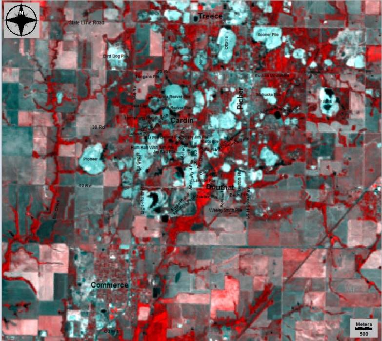
From here to the end of this page, titles for images involving rollovers will be typed rather than included on the images so that images are easier to match in shape for rollovers. Next is a composite of 2, 3, 4 for years 1988 and 2010. These two images were used for reference often due to the amount of vegetation in the images.
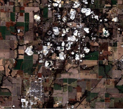
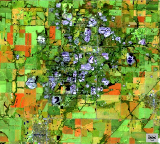
Composite of Bands 2, 3, and 4, color-coded Blue, Green and Red
12/9/88 first image 12/6/10 second image
Click here for larger 1988 image Click here for larger 2010 image
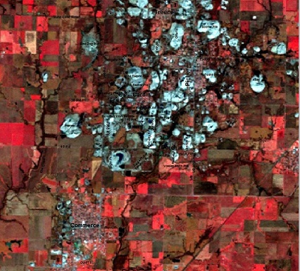
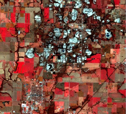
In the traditional false-color composite, created with bands 2, 3, 4, deep water is black and dark grey and shallow and sediment-laden water is in lighter shades of grey. Notice the slight difference in color in the two pools at the Picher water treatment plant on the east edge of the 2010 image. This could be due to differing depth in the pools but is likely due to differences in suspended sediment content as well. To the northeast of the crescent shape in the 2010 image, it is noticeable that the water body is larger in 2010 than in the 1988 image. Notice the change in shape of the Atlas chat pile from 1988 to 2010. There are more areas in the pile with pools of water in the 2010 image. There are a lot of differences in the use for land plots--as there are fields with active vegetation in one image while there are a lot of different fields with active vegetation in the other image. The brightest red plots with vegetation are likely primarily winter wheat fields. While not existent in the 1988 image, the OU Passive Treatment System (PTS) is visible in the 2010 image in the community of Commerce. It is in light shades of grey, either an indication of shallow water or sediment. The southeastern part of the PTS is lighter, so it is even more shallow or filled with sediment. Two of the furthest eastern pools contain limestone which might account for the lighter hue (observation). Also, notice the coloration of the pools at Domado and Skelton tailings piles. The pools at the tailings piles appear paler blue-grey and are known to be laden with metals. There is also a circular shape of lighter teal above the word Douthat (the former mining community in the area). This area is an area of known mine collapse. Dr. Luza noted this area actually contains six collapses. Much wetland vegetation is forming--even beavers have moved in. The pool is either heavy in metals, sediment, both, or is shallow.
In the composite, the waters along Tar and Lytle creeks appear to be shallow or sediment-laden in many areas and slightly deeper in a few small areas (the dark grey-to-black color). The waters below Bird Dog pile and on southwestward in the waters of Elm Creek do not display purely as water in the composites. This is partially due to heavy riparian vegetation in shades of reddish-brown along the streams this time of year (December). The mix of vegetation and water creates a muddied, dull tone along some of the stream and yet some deeper areas of water are still evident in shades of grey. Notice the difference in the coloration of the unnamed tributary of Elm Creek that trends southwest below Bird Dog tailings pile and that of Elm Creek. Part of this difference in color is due to differences in depth and sediment--it is a smaller stream. However, there is also more grey shading which could be due to chat and fines in the stream close to 20 Road. Healthy vegetation is bright red in this combination and chat piles are in various shades of grey to white.
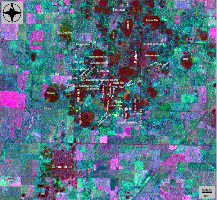
Due to the unusual coloration of the August 3, 2011 composite for Bands 2, 3, and 4, also color-coded blue, green and red, it is included below:
Click here for larger image of composite.
Marked differences are noted between the 2011 composite for bands 2, 3, and 4 and the 1988 and 2010 composites likely due to winter wheat harvested in June/July and the drought conditions experienced in the summer of 2011. In comparing the false color composites, one will note the red coloration is much more vivid and prevalent in fields, likely due to crops in the 2010 image, indicating much more active, healthy vegetation. However, in the August 2011imagery, even after the effects of drought, active riparian vegetation is noticeable along Elm Creek, Tar Creek and around chat piles, for instance in Picher between Sooner and Mahuska tailings piles. To note, however, there are also many bare and fallow land plots in the 2011 image. Interestingly, the chat piles have more of a cyan tint in the 2011 image, likely an indication there is less water stored within the chat piles after the drought period and more perception of the signature of chat rather than chat mixed with water (a more greyish tone).
Between years, there are also differences in the coloration of the water, for instance at the Picher water treatment plant pools. There is a much more noticeable difference in water color between the two pools in the 2011 image (notice the more southeastern pool), either indicating a difference in depth or content of the pools.
Landsat composites of bands 1, 5, 4 were also created for 1988, 2010 and 2011.
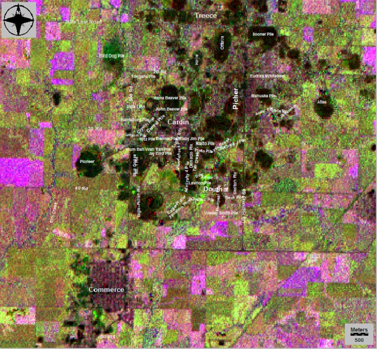
Composite of Bands 1, 5, and 4 (color coded blue, green, red)
12/9/88 first image 12/6/10 second image

Click here for larger 1988 image Click here for larger 2010 image
Riparian vegetation is emphasized in the 2010 image, especially around the chat piles and along the creeks. The chat coloration in the 2011 composite was so unusual that Principal Components Analysis (PCA) was warranted for the imagery. PCA is a linear transformation technique related to factor analysis. Given the set of image bands, PCA produces a new set of imges that are uncorrelated with one another and are ordered in terms of the amount of variance they explain from the original band set. PCA was recommended in the paper, The Use of Remote Sensing Technology in geological Investigation and mineral Detection in El Azraq-Jordan, for the first five bands. As I was not needing Band 2, I only ran the module for bands 1, 3, 4, and 5. Note, the date of the imagery is actually 8-03-11-the file names below reflect an error by the author in naming the files. After running the PCA module, the table generated by the module was examined (see below):
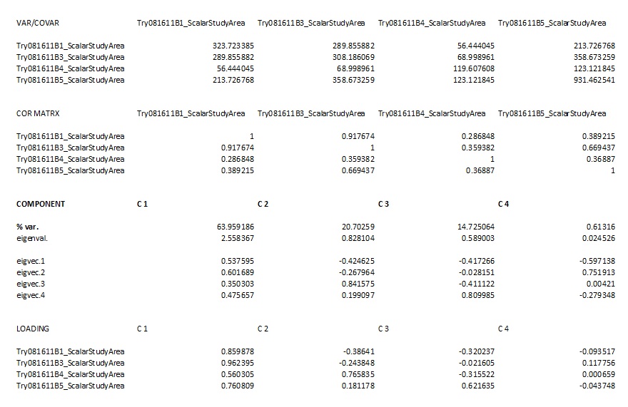
Notice under the category Component % Var., the majority of the information was contained in bands 1, 3, and 4. In considering this, I next ran the inverse PCA module, omitting the final band and then prepared the composite again for the August 2011 Bands 1, 5 and 4, using the inverse PCA bands for 1 and 4. The differences between the original composite and new bands are minor at best and actually difficult to pinpoint.
Composite of Bands 1, 5, and 4 for August 2011 (color coded blue, green, red)
August 3, 2011 first image August 3, 2011 Composite with Inverse PCA

Click here for larger 2011 image Click here for larger 2011 Inverse PCA image
Healthy vegetation is in shades of orange rather than in the standard false-color composite’s shades of red. There is little active vegetation in cropland in the 2011 composite due to the summer 2011 drought. The band 1, 5, 4 combination displays the study areas’ deep and clear water in deepest blue and more shallow water or sediment-laden water in various shades of lighter blue. Interestingly, in this combination, the chat piles contain much more blue shading in the 2011 composites. The sensitivity of the mid-infrared band to water is likely the reason for the increase in blue shading in the chat piles and indicates there is likely still water within the piles. Notice the deeper blue in the Anna Beaver pile and lavender in the Mahuska pile. Ken Luza, Oklahoma University, noted the Anna Beaver pile is one of the largest, and so the deep coloration is likely due to more water stored in the pile.
Since this was during a drought, this observation would suggest more water such as during periods of normal rainful likely results in shades of grey in the color of the piles and obscures the spectral signature of the chat alone. This line of thinking makes sense as the same piles are more of a bluish-grey in the December composites. More areas of shallow or sediment-laden water are obvious in this composite for all three years which allows one to compare the same areas in the traditional composite and realize some areas that did not appear to be water are either shallow water or sediment-laden water. This composite clearly shows water in varying depths around the bases of chat piles and indicates there is water in the chat piles as well. As with the Band 2, 3 and 4 composite for 2011, the 1, 5 and 4 composite for 2011 again emphasized the difference in color between the two water treatment pools in Picher.
The false color composites emphasize small ponds of water that are not visible in the natural color image. The August false color composites emphasize a significant amount of riparian vegetation surrounding a number of tailings piles which indicates substantial flow of water from the piles. All of the composites accentuate the water-filled depression areas in the Atlas tailings pile and the crescent shaped area of water below 40 Road. There appears to be more sediment or shallow depth in the southwestern edge of the pond of water to the west of Admiralty 4 tailings pile (northeast of the crescent shape), due to the lighter coloration of the water in the Landsat composites. Looking at the natural color composites (Bands 1, 2, and 3) for accuracy assessment, the coloration is lighter in the same area but it is not obvious that the area is water. One benefit of the false-color Landsat composites is that spectral signatures aid in identification.
The Taiga Overlay module is located within the GIS Analysis/Database Query Tabs. Using the Idrisi Taiga Overlay module, band ratios were prepared of the December 9, 1988 and December 6, 2010 cropped datasets.
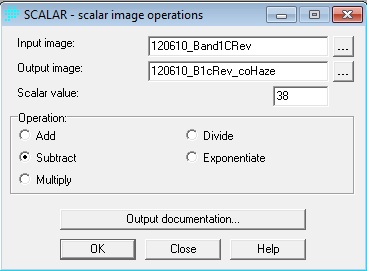
Prior to preparing the ratios, haze correction was performed using the Taiga Scalar module. Both modules are mathematical operators.
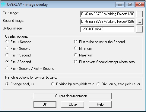
Band ratio composites prepared included a composite of band ratios 5/7-3/1-4/5 and a composite of band ratios 4/3-3/1-5/7. The natural color composite of Bands 1, 2, and 3 for the respective datasets were again used for accuracy assessment.
Composite of Band Ratios 5/7-3/1-4/5
12/9/88 first image 12/6/10 second image
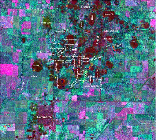
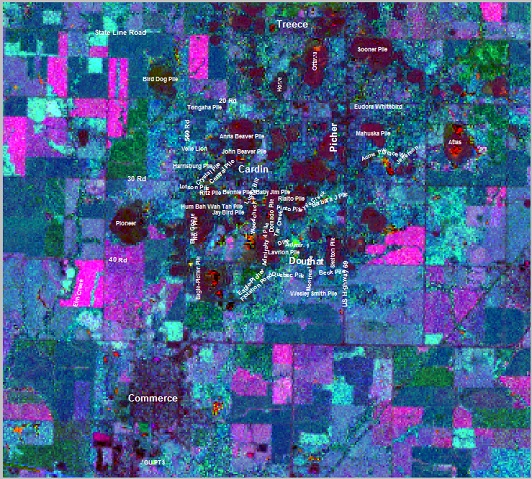
Click here for larger 1988 image Click here for larger 2010 image
In the composite with band ratios 5/7, 3/1, 4/5 (color coded blue, green, red), the image emphasizes differences in color within the chat piles. Notice the differences in color in the Bird Dog tailings pile and Sooner tailings pile. Bird Dog has little remaining chat, but a large amount of flotation pond slimes mixed with fines-a condition not found at most other piles and a likely reason for the variation in color since slimes and fines are higher in metals content than chat and likely have different reflective qualities and spectral signature as well. The basin below Bird Dog pile (below 20 Rd) picks up a lot of green color but it appears in satellite imagery to have some small deposits of waste rock and/or fines in the basin which could account for the coloration. The bright green area toward the top of the Eagle-Picher Flotation pond below 40 Rd is a vegetated area within the fines. Notice the differences in the water colors in the water treatment plants and the water-filled depression (crescent shape). There are also variations in color in the pools at the treatment plants in Picher and Commerce. Notice there is an increase in water-filled depressions at Atlas pile in the 2010 image.Water is evident at the north of Ottawa pile in the 2010 image but is not evident in the 1988 image. The variation in color in the Atlas tailings pile is due to a number of water-filled depressions with varying depths or amounts of sediment. Ken Luza, Oklahoma University of Oklahoma, noted the water in the crescent shaped area below 40 Road and in Atlas pile are not from collapses, but rather simply areas of depression in the chat. The primary confirmation from this ratio composite is that the contents at Bird Dog pile are different than at most of the piles. Green coloration in the Bird Dog pile could possibly indicate higher iron-oxide content in the pile.
Composite of Band Ratios 4/3-3/1-5/7
12/9/88 first image 12/6/10 second image
Click here for larger 1988 image Click here for larger 2010 image
In the composite with band ratios 4/3-3/1-5/7 (color coded blue, green, red) the image was prepared in an attempt to recognize hydrothermally altered bedrock, since much of the ore emplacement is thought to be related to hydrothermal deposits (Vandeberg, 2003). Notice that the chat piles are mostly green or green mixed with brown color, which indicates band combination 3/1 is dominating the image. This implies a high iron-oxide content in the tailings pile signature (Vandeberg, 2003). Notice the difference in coloration of Bird Dog tailings pile (mostly green) and Sooner Pile (mostly brown).There appears to be more fields of active vegetation in the 2010 composite of ratios than in the 1988 composite, and water color differs between years as well.
Both varieties of band ratio composites appear speckly. Ratios tend to enhance noise or small-spatial variations and the noise is emphasized even further when composites are prepared with three ratios (Aber, J.S. conversation). Even so, this method definitely brought out otherwise understated variances in the chat piles.
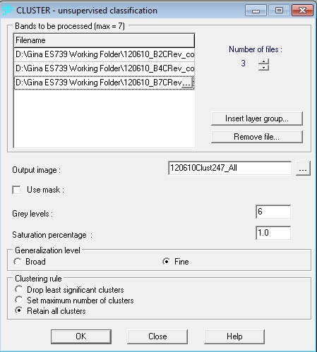
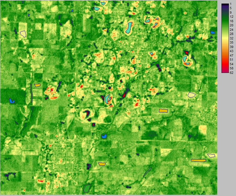
Additionally, Landsat satellite imagery was used for cluster analysis and change analysis. According to the Idrisi Taiga manual, the cluster module performed unsupervised classification based on the set of input images using a multi-dimensional histogram peak technique. It is run from the Image Processing/Hard Classifiers menu. Using Taiga’s Cluster module an analysis was conducted of December 1988 and December 2010 Landsat imagery for Bands 2, 4 and 7.
The initial analysis resulted in 24 clusters for the December 1988 imagery and 36 clusters for the December, 2010 imagery. Looking at the histogram for each resulting image, it was clear that almost all of the data variation was depicted in many less clusters so the images were reclassified by running the Cluster module again with less clusters:
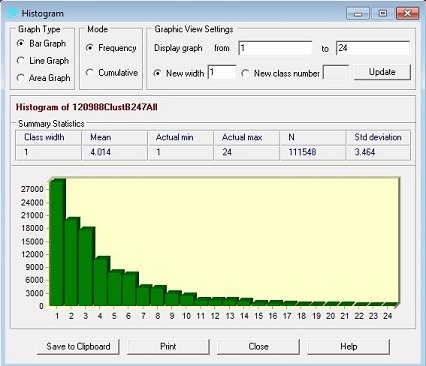
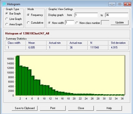
The analysis was rerun with 8 clusters for the 1988 image bands and 11 clusters for the 2010 image bands due to the drop offs in the histograms.
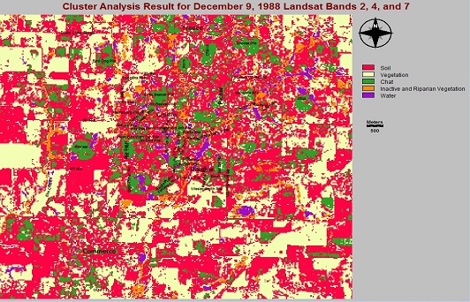
The second effort for the December 9, 1988 Cluster Analysis of Landsat Imagery with eight clusters resulted in clusters for soil, soil, vegetation, vegetation, chat, inactive and riparian vegetation, vegetation and water. Due to redundant clusters, the edit and assign programs were again used as above to assign five clusters in the final image. The final result for 1988 cluster analysis follows (click on image for larger view):
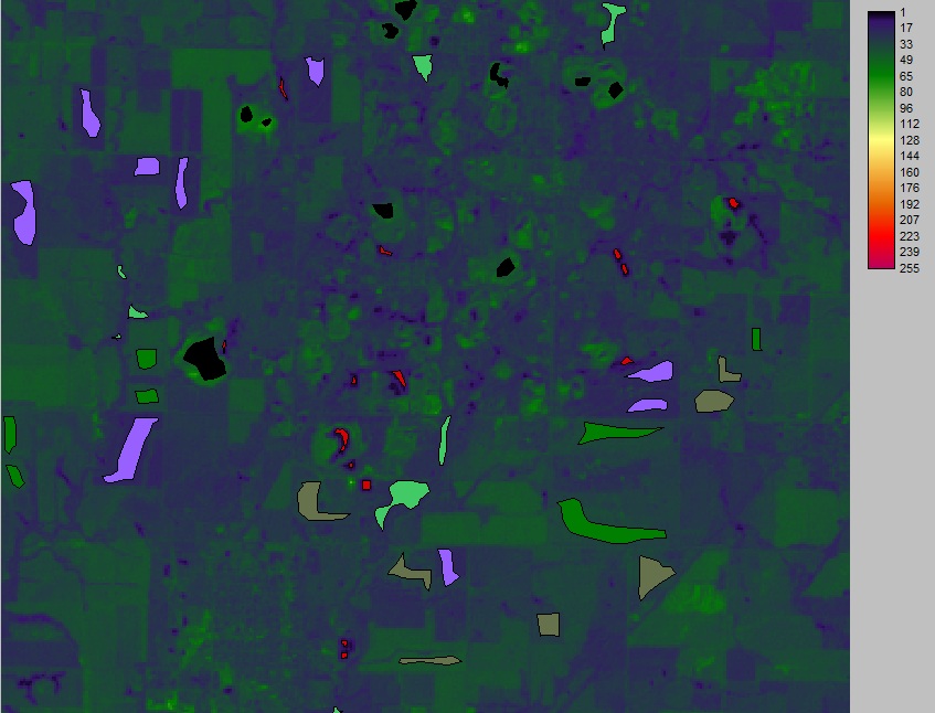
The second effort for the December 6, 2010 Cluster Analysis of Landsat Imagery with 11 clusters resulted in clusters for inactive and riparian vegetation, fallo field or soil, vegetation, vegetation, soil, chat, vegetation, fallow field or soil, vegetation, vegetation, and water. As with the 1988 imagery, due to redundant clusters for the 2010 analysis, the edit and assign programs were again used as above to assign six clusters in the final image. The final result for 1988 cluster analysis follows (click on image for larger view):
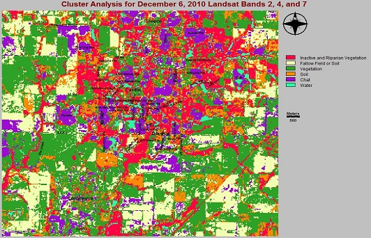
Results were fairly accurate with the exception of the amount of chat in the community of Commerce. It is possible some urban structures in the community are classified as chat.. There is a noticeable increase in riparian vegetation between the years of 1988 and 2010 which is a logical change since the chat piles serve as an aquifer and wetlands are forming in the area.
Next, interactive screen digitizing was utilized as a means for delineating training sites to prepare for supervised classification of the 1988 and 2010 imagery.
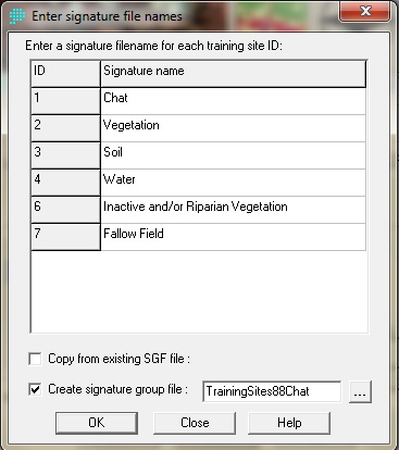
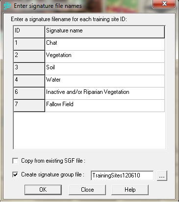
To create training sites for the respective years, polygons were created for each primary feature. Training sites were pinpointed for chat, vegetation, soil, water, inactive and/or riparian vegetation and fallow fields.
View 1988 Training Sites here and view 2010 training sites here.
Next, signature files were created. Signature files contain statistical information about the reflectance values of the pixels within the training sites for each class. To create signature files for each year, the MAKESIG module from the Image Processing/Signature Development menu is utilized.
To verify creation of the signature files, the filter for signature files and signature groups was checked and it was verified that the files were all available within Explorer.
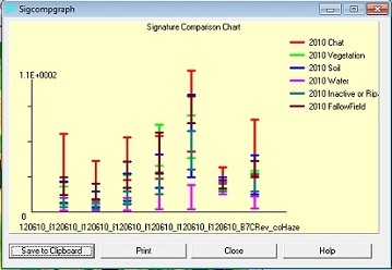
Next, the module, SIGCOMP from the Image Processing/Signature Development menu was utilized for viewing of means for the signatures in the different bands.

The following step was to classify the images based on these signature files. Each pixel in the study area has a value in each of the bands of imagery. These values mesh to form a unique signature which can be compared with the prepared signature files.
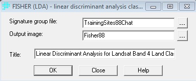
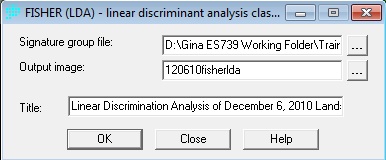
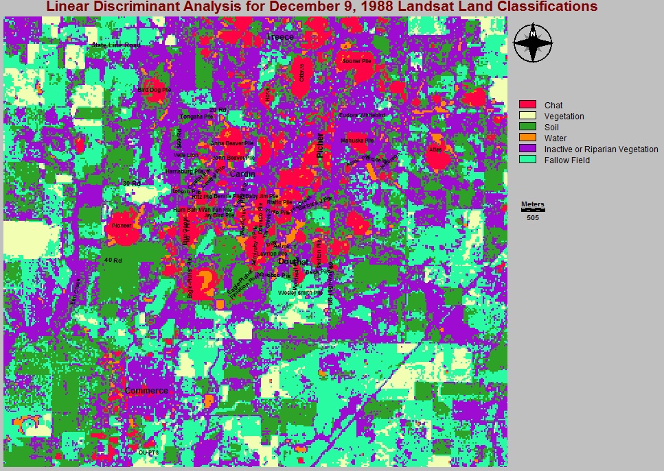
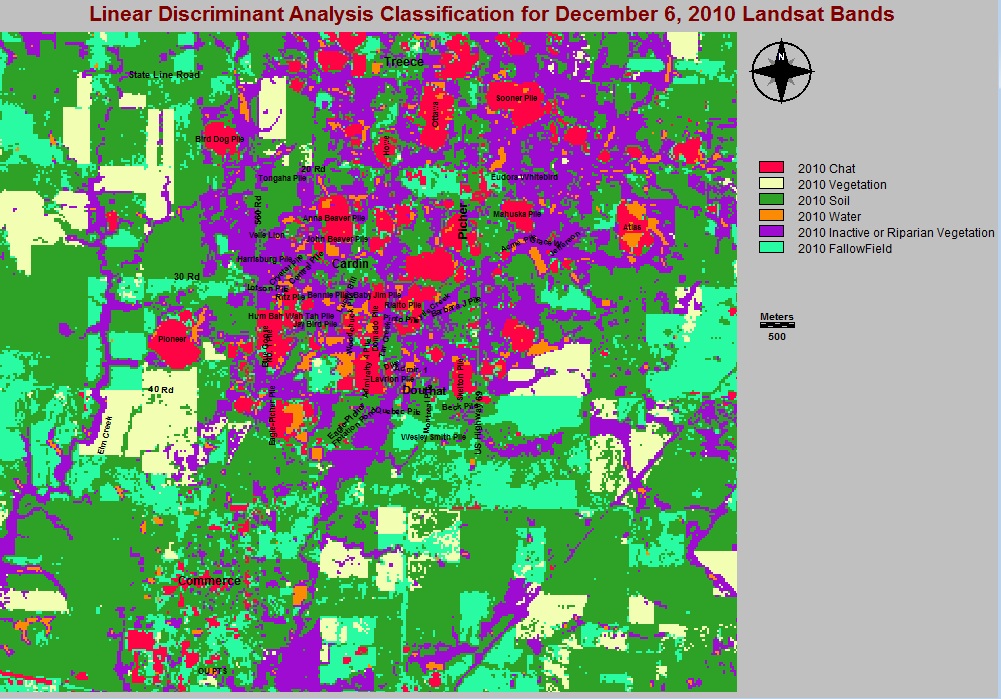
Using the signature files created, supervised classification was conducted using the Fisher Linear Discriminant Analysis (LDA) module for both years:
The FISHER classifier conducts a linear discriminant analysis of the training site data to arrange a set of linear functions that define the degree of support for each class. The assigned class for each pixel is then the class that obtains the greatest support after evaluation of all functions. These functions have a form similar to that of a multivariate linear regression equation, with independent variables as the image bands, and the dependent variable as the measure of support. It was stressed in the Idrisi Manual that equations are calculated in a manner that maximizes the variance between classes and minimizes variance within classes. According to the manual, the number of equations will be equal to the number of bands, each describing a hyperplane of support. The intersections of these planes then form the boundaries between classes in band space.
To view Fisher LDA results for the 1988 Landsat imagery click here.
To view FISHER LDA results for the 2010 Landsat imagery click here.
The LDA classification successfully identified water at the Oklahoma University Passive Treatment System in the 2010 imagery-a definite improvement over unsupervised classification for identifying small, shallow water features.
Subsequently, the Idrisi Land Change Modeler was utilized for comparision of the FISHER LDA 1988 and 2010 images. The portion of the Land Change Modeler that was utilized in this project is intended for the integrated analysis of landcover change. Two images containing, at a minimum, either unsupervised or supervised classification from two different dates are required for the modeler to run most of the module's features..
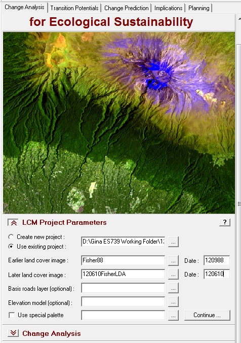
Next, the change analysis tab was accessed and gains and losses by category between the years was determined in km2
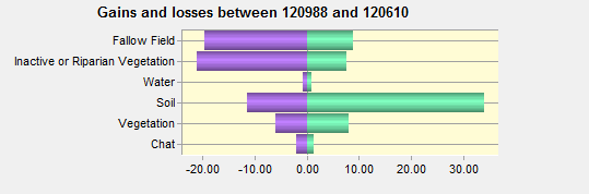
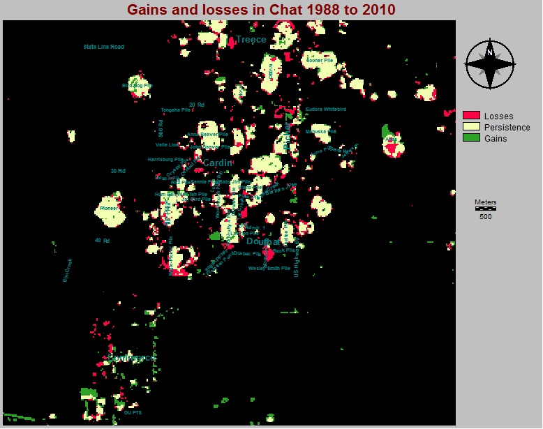
Also, the tab for gains and losses for chat was selected:
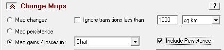
To see the resulting map for this module click here. This amount of change seems reasonable.
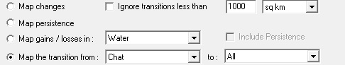
The tab for gains and losses for water was purposely selected due to interest in seeing if the module again pinpoints the water at the OU PTS in the 2010 image:
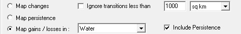
To see the resulting map for this module click here. Again, with the use of the Fisher linear discriminant analysis, the water was accurately detected as a gain at the OU PTS. There is an area of water loss to the northeast of the dike to the east of Admiralty 4 tailings pile. The dike was constructed in an effort to divert Lytle Creek runoff to Tar Creek and the coloration indicates the effort has worked to some extent.
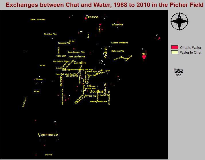
Additionally, the tab for exchanges between chat and water was selected.
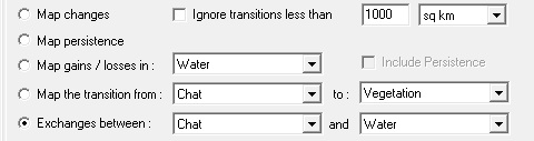
To see the resulting map for this module click here.
Notice the results for Atlas chat pile. The exchanges between water and tailings is logical since there are several areas of water that have developed in the pile. The chat to water and water to chat areas to the west of Admiralty 4 tailings pile are likely within the Quapaw Tribe’s chat washing operation.
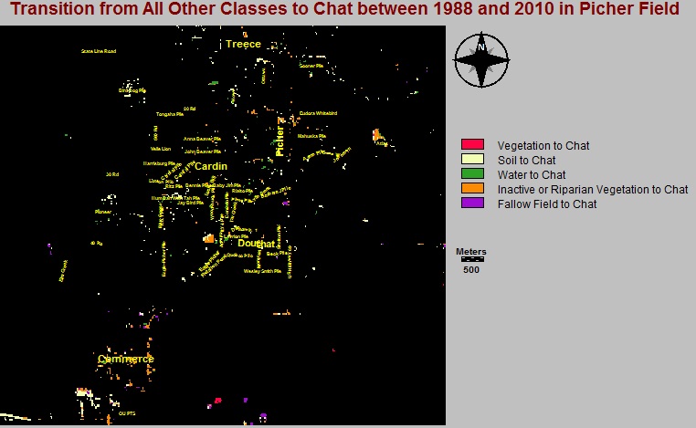
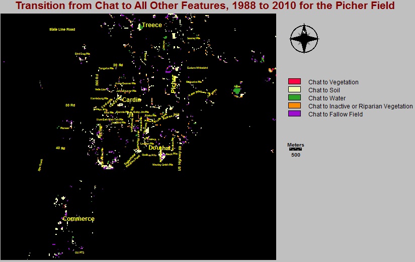
Moreover, the tabs for transition from all other signatures to chat and for transition from chat to all other signatures were selected:
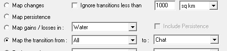
To see the resulting map for these features click here and here. Again, notice the changes at Atlas chat pile.
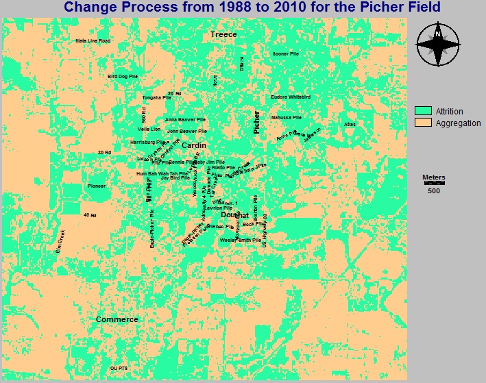
Lastly, the change process was analyzed using the same two images. To access the change process feature, click on the Implications tab, then the landscape pattern and change process analysis tab.
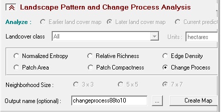
The Change Process option compared the 1988 and 2010 landcover maps and measured the nature of the change underway within each landcover class. This is conducted through use of a decision tree procedure that compares the number of landcover patches present within each class between the two time periods to changes in their areas and perimeters. The output is in the form of a map. Landcover classes are assigned the category of change that are experiences.
To see the resulting map for this module click here. The interpretation of the categories of change that were identified follows:
Attrition indicates the number of patches and the area are decreasing; aggregation indicates the number of patches is decreasing but area is constant or increasing. With the amount of activity taking place during remediation, the results for this feature were rather surprising since only two types of change were identified by the process for Picher Field. Overall, the processes used in this project were successful in pinpointing variabilities and changes in the landscape.
Problems with this webpage? Please
click here to
notify author. Thank you.
© Gina Manders, 2011